Both Shannon et al. [1], [2] and Kolmogorov-Chaitin–Solomonoff (KCS)1 [2] [3] [4] [5] [6] [7] [8] [9] measures of information are famous for not being able to measure meaning. A DVD containing the movie Braveheart
and a DVD full of correlated random noise can both require the same
Shannon information as measured in bytes. Likewise, a maximally
compressed text file with fixed byte size can either contain a classic
European novel or can correspond to random meaningless alphanumeric
characters. The KCS measure of information is therefore also not able
to, by itself, measure informational meaning.
We propose an information theoretic method to measure meaning [10], [11].
Fundamentally, we model meaning to be in the context of the observer. A
page filled with Kanji symbols will have little meaning to someone who
neither speaks nor reads Japanese. Likewise, a machine is an arrangement
of parts that exhibit some meaningful function whose appreciation
requires context. The distinguishing characteristic of machines is that
the parts themselves are not responsible for the machine’s
functionality, but rather they are only functional due to the particular
arrangement of the parts. Almost any other arrangement of the same
parts would not produce anything interesting. A functioning
computational machine is more meaningful than a large drawer full of
computer parts. We appreciate the meaningful functionality of the
machine only because we have the contextual experience to recognize what
the machine can do or is capable of doing.
The arranging of a large collection of parts into a working machine is highly improbable. However, any
arrangement would be improbable regardless of whether the configuration
had any functionality whatsoever. For this reason, neither Shannon nor
KCS information models are capable of directly measuring meaning.
Functional machines are specified—they follow some independent pattern.
When something is both improbable and specified, we say that it exhibits
specified complexity. An elaborate functional machine
exemplifies high specified complexity. We propose a model, algorithmic
specified complexity (ACS), whereby specified complexity can be measured
in bits.
ASC was introduced by Dembski [12]. The topic has been developed and illustrated with a number of elementary examples [10], [11]. Durston et al.’s functional information model [13] is a special case. The approach differs from conventional signal and image detection [14] [15] [16] [17] [18] [19] including matched filter correlation identification of the index of one of a number of library images [20] [21] [22].
Alternately, ACS uses conditional KCS complexity to measure the minimum
information required to reproduce an image losslessly (i.e., exactly -
pixel by pixel) in the presence of context. Use of KCS complexity has
been used elsewhere to measure meaning in other ways. Kolmogorov sufficient statistics [2], [23]
can be used in a two-part procedure. First, the degree to which an
object deviates from random is ascertained. What remains is
algorithmically random. The algorithmically nonrandom portion of the object is then said to capture the meaning of the object [24].
The term meaning here is solely determined by the internal structure of
the object under consideration and does not directly consider the
context available to the observer as is done in ASC.
A. Game of Life
To illustrate quantitative measurement of specified complexity, we examine the well-defined universe of Conway’s Game of Life [25].
In the Game of Life, a 2-D grid of living and dead cells live and die
based on simple rules. At each time step a cell is determined to be
alive or dead depending on the state of its neighbors in the previous
generation.
Within the Game of Life, interesting and elaborate forms have been
discovered and invented. These are particular arrangements of living and
dead cells that when left to operate by the rules of the game, exhibit
meaningful functionality. Some oscillate, some move, some produce other
patterns, etc. Some of these are simple enough that they arise from
random configurations of cell space. Others required careful construction, such as the very large Gemini [26].
Our goal is to formulate and apply specified complexity measures to
these patterns. We would like to be able to quantify what separates a
simple glider, readily produced from almost any randomly configured
soup, from Gemini—a large, complex design whose formation by chance is
probabilistically minuscule. Likewise, we would like to be able to
differentiate the functionality of Gemini from a soup of randomly chosen
pixels over a similarly sized field of grid squares.
A highly probable object can be explained by randomness, but it will
lack complexity and thus not have specified complexity. Conversely, any
sample of random noise will be improbable, but will lack specification
and thus also lack specified complexity. In order to have specified
complexity, both components must be present. The object must exhibit a
describable functioning pattern while being improbable.
Our paper differs from the study of emergence in cellular automata first proposed by von Neumann [27], [28] for investigating self-reproduction. The study of dynamic cellular automata properties, popularized by Wolfram [29], deals largely with investigation of the temporal development of emergent behavior [30].
As an example, the set of all initializations that lead to the same
emergent behavior, dubbed the basin of attraction, has been studied as a
model for evolution of artificial life with application to the modeling
of memory and neural networks [30] [31] [32] [33]. Akin to biological swarms obeying simple nonlinear rules [34] [35] [36], emergence is difficult to predict thereby necessitating largely experimental analysis.
Our paper, in contrast, deals with measuring meaning in existing objects. In assessing the specified complexity of Braveheart
versus the DVD of noise, we are not interested in finding the dynamics
of where each DVD came from but, rather, how we assess what has meaning
and what does not. It is in this context that we deal with assessment of
specified complexity of the Game of Life.
SECTION II
ALGORITHMIC SPECIFIED COMPLEXITY
How does one measure specification? One possibility is to use KCS complexity [4], [5], [9]. An introduction to the topic is in the widely used information theory text by Cover and Thomas [2]. A more advanced presentation is given by Li and Vitâanyi [23]. KCS complexity or variations thereof have been previously proposed as a way to measure specification [12], [37], [38].
KCS complexity is defined as the length of the shortest computer program,  $p$, in the set of all programs,
  $P$, that produces a specified output
  $X$ using a universal Turing machine,
  $U$
$U$ TeX Source$$\begin{equation*} K(X) = \min _{U(p,) = X | p\in P} |p|. \end{equation*}$$ Such programs are said to be elite [8]. Conditional KCS complexity [3] allows programs to have input,
  $Y$, which is not considered a part of the elite program
  TeX Source$$\begin{equation*} K(X|Y) = \min _{U(p,Y) = X | p\in P} |p|. \end{equation*}$$ For our purposes,
  $Y$ can be considered as context.
An example is Shakespeare’s Hamlet compressed with two different resources: 1)  $Y_{\rm alpha} =$ the English alphabet, including numbers and punctuation and 2)
  $Y_{\rm con} =$ an exhaustive concordance of the words used in all of Shakespeare’s writings [39]. Both resources can be viewed as a code book in which the entries are lexicographically listed and numbered. Hamlet, corresponding to the output
  $X$,
can then either be expressed as a sequence of integers each
corresponding to an entry in the alphabet list, or indexed as an entry
in the concordance. Shakespeare used 31534 different words [40]. Although both the alphabet and concordance characterizations bound the conditional KCS complexity, we would expect
$X$,
can then either be expressed as a sequence of integers each
corresponding to an entry in the alphabet list, or indexed as an entry
in the concordance. Shakespeare used 31534 different words [40]. Although both the alphabet and concordance characterizations bound the conditional KCS complexity, we would expect  TeX Source$$\begin{equation*} K\left (X|Y_{con}\right )<K\left (X|Y_{alpha}\right )<K(X). \end{equation*}$$
The more specific the context, the smaller the elite program. Either
the frequency of occurrence of the words used by Shakespeare or a
concordance of words used only in Hamlet can be used to reduce
the conditional KCS complexity even further. Small conditional KCS
complexity can be caused by the following.
- Placing
 $X$ in the context of
  $Y$ and/or
- A small (unconditional) KCS complexity,
 $K(X)$.
A small value of  $K(X|Y)$ can therefore arise from the small complexity of
  $X$ and/or from the available context,
  $Y$.
$Y$.
A. ASC: Actual and Observed
Algorithmic specified complexity [41] is defined as  TeX Source$$\begin{equation*} ASC(X,C,P) = I(X) - K(X|C)\tag{1}\end{equation*}$$ where
 $X$ is the object or event under consideration;
 $C$ is the context (given information) which can be used to describe the object;
 $K(X|C)$ is the KCS complexity of object
  $X$ given context
  $C$;
$C$; $P(X)$ is the probability of
  $X$ under the given stochastic model;
 $I(X) = -\log _{2} \left ( P(X) \right )$ is the corresponding self information.
The ASC measure bears a resemblance to both Shannon [1], [2] and KCS [23] mutual information.
ASC is probabilistically rare in the sense that [42] TeX Source$$\begin{equation*} \Pr \left [ ASC(X,C,P) \geq \alpha \right ] \leq 2^{-\alpha }.\tag{2}\end{equation*}$$ For example, the chance of observing ten or more bits of ASC does not exceed
  $2^{-10}\approx$ one chance in a thousand. ASC provides evidence that a stochastic outcome modeled by the distribution,
  $P(X)$, does not explain a given object. ASC is incomputable because KCS complexity is incomputable [2].
However, the true KCS complexity is always equal to or less than any
achieved lossless compression. This means that the true ASC is always
equal to or more than an estimate. We will refer to the known estimate
as the observed observed algorithmic specified complexity (OASC). We
know that
$P(X)$, does not explain a given object. ASC is incomputable because KCS complexity is incomputable [2].
However, the true KCS complexity is always equal to or less than any
achieved lossless compression. This means that the true ASC is always
equal to or more than an estimate. We will refer to the known estimate
as the observed observed algorithmic specified complexity (OASC). We
know that  TeX Source$$\begin{equation*} ASC(X,C,P) \geq OASC(X,C,P).\tag{3}\end{equation*}$$
The inequality in (2) applies to OASC. From (3), we conclude there is a  $k \geq 0$ such that 2
 TeX Source$$\begin{equation*} OASC = ASC - k. \end{equation*}$$ Thus
 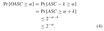 TeX Source$$\begin{align*}
\Pr \left [OASC \geq \alpha \right ]=&\Pr [ASC - k \geq \alpha ]
\\=&\Pr [ASC \geq \alpha + k]\\&\leq 2^{-\alpha - k}\notag
\\&\leq 2^{-\alpha }.\tag{4}\end{align*}$$ OASC therefore obeys the same bound as does ASC in (2).
TeX Source$$\begin{align*}
\Pr \left [OASC \geq \alpha \right ]=&\Pr [ASC - k \geq \alpha ]
\\=&\Pr [ASC \geq \alpha + k]\\&\leq 2^{-\alpha - k}\notag
\\&\leq 2^{-\alpha }.\tag{4}\end{align*}$$ OASC therefore obeys the same bound as does ASC in (2).
ASC can be nicely illustrated using various functional patterns in Conway’s Game of Life. The Game of Life and similar systems allow a variety of fascinating behaviors [29].
In the game, determining the probability of a pattern arising from a
random configuration of cells is difficult. The complex interactions of
patterns arising from such a random configuration makes it difficult to
predict what types of patterns will eventually arise. It would be
straightforward to calculate the probability of a pattern arising
directly from some sort of random pattern generator. However, once the
Game of Life rules are applied, determining what patterns would arise
from the initial random patterns is nontrivial. In order to approximate
the probabilities, we will assume that the probability of a pattern
arising is about the same whether or not the rules of the Game of Life
are applied, i.e., the rules of the Game of Life do not make interesting
patterns much more probable then they would otherwise be.
Objects with high ASC defy explanation by the stochastic process
model. Thus, we expect objects with large ASC are designed rather than
arising spontaneously. Note, however, we are only approximating the
complexity of patterns and the result is only probabilistic. We expect
that patterns requiring more design will have higher values of ASC.
Smaller designed patterns exist, but it is not possible to conclude that
they were not produced by random configurations.
Section III documents the methodology of the
paper. We define a mathematical formulation to capture the functionality
of various patterns. This can be encoded as a bitstring and a program
written to generate the original pattern from this functional
description. Section IV uses this methodology to calculate ASC for a variety of patterns found in the Game of Life.
A. Specification
The Game of Life is played on grid of square cells. A cell is either
alive (a one) or dead (a zero). A cell’s status is determined by the
status of other cells around it. Only four rules are followed.
- Under-Population: A living cell with fewer than two live neighbors dies.
- Family: A living cell with two or three live neighbors lives on to the next generation.
- Overcrowding: A living cell with more than three living neighbors dies.
- Reproduction: A dead cell with exactly three living neighbors becomes a living cell.
As witnessed by videos on YouTube, astonishing functionality can be achieved with these few simple rules [43] [44] [45].
If the reader is unfamiliar with the diversity achievable with these
operations, we encourage them to view these and other short videos
demonstrating the Game of Life. The static pictures in this paper do not
do justice to the remarkable underlying dynamics. There is also an active users group [46].
The rules for the Game of Life are deterministic. Performance is
therefore dictated only by the initially chosen pattern. In order to
demonstrate the compression of functional Game of Life patterns, we
first devise a contextual mathematical formulation for describing
functionality. A method for interpreting this formulation is considered
to be part of the context. Let  $X$ be some arbitrary pattern corresponding to a configuration of living and dead pixels. Let
  $X\oplus$ be the result of one iteration of the Game of Life applied to
  $X$. Suppose that the following equality holds:
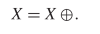 TeX Source$$\begin{equation*} X = X \oplus \!. \end{equation*}$$ This says that a pattern does not change from one iteration to the next. This is known as a still-life [25], and an example is presented in Fig. 1. A more interesting pattern can be described as
 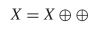 TeX Source$$\begin{equation*} X = X \oplus \oplus \end{equation*}$$
which can be a pattern that returns to its original state after two
iterations. The relationship is also valid for two iterations of a
still-life. In order to differentiate a two-iteration flip-flop from a
still life form, two equations are required
TeX Source$$\begin{equation*} X = X \oplus \oplus \end{equation*}$$
which can be a pattern that returns to its original state after two
iterations. The relationship is also valid for two iterations of a
still-life. In order to differentiate a two-iteration flip-flop from a
still life form, two equations are required 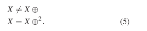 TeX Source$$\begin{align*} X\neq&X \oplus \notag \\ X=&X \oplus ^{2}.\tag{5}\end{align*}$$
We often need to specify that a rule holds only for some parameter and
not for any smaller version of that. We therefore adopt the notation
TeX Source$$\begin{align*} X\neq&X \oplus \notag \\ X=&X \oplus ^{2}.\tag{5}\end{align*}$$
We often need to specify that a rule holds only for some parameter and
not for any smaller version of that. We therefore adopt the notation 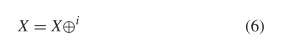 TeX Source$$\begin{equation*} X = X \oplus ^{i}\tag{6}\end{equation*}$$ to mean a pattern that repeats in
  $i$ iterations, but not in less than
  $i$ iterations. An example for
  $i = 2$, shown in Fig. 2, is a period-2 oscillator [46] or a flip-flop [25].
One of the more famous Game of Life patterns is the glider. This is a
pattern which moves as it iterates. A depiction is shown in Fig. 3. In order to represent movements we introduce arrows, so  $X\uparrow$
is the pattern X shifted up one row. Since four iterations regenerate
the glider shifted one unit to the right and one unit down, we can write
$X\uparrow$
is the pattern X shifted up one row. Since four iterations regenerate
the glider shifted one unit to the right and one unit down, we can write
 TeX Source$$\begin{equation*} X\downarrow \rightarrow = X \oplus ^{4}\!.\tag{7}\end{equation*}$$ This defines the functionality of moving in the direction and speed of the glider.
We can also simply insert a pattern into the mathematical
formulation. For the simplest case, we can say that the pattern is equal
to a particular pattern. For example
Note that to the right of the equals sign here is a small picture of the glider in Fig. 3. We can also combine patterns, for example taking the union
or the intersection
We can also describe a pattern as the set-difference of two other patterns. Since  $A \smallsetminus B$ denote elements in
  $A$ not in
  $B$, we have for example
At times, it may be useful to define variables. For example 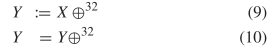 TeX Source$$\begin{align*} Y ~:\!\!=&X \oplus ^{32}\tag{9}\\ Y =&Y \oplus ^{32}\tag{10}\end{align*}$$ where
  $: =$ denotes “equal to by definition.” This reduces to
  TeX Source$$\begin{equation*} X\oplus ^{32} = X \oplus ^{64}\!. \end{equation*}$$
Table I provides a listing of operations. The
selected set of operation was chosen in attempt to cover all bases which
might be useful, but is still arbitrary. Another set of operations with
more or less power could be chosen. By using a consistent set of
operations between the various examples explored in this paper, we
obtain comparable OASC values.
More that one  $X$ will display two step oscillation in accordance to
  $X = X \oplus ^{2}$.
In fact, this and other equations will admit an infinite set of
patterns that satisfy the description. In order to make an equation
description apply to a unique pattern, we can lexicographically order
all patterns obeying a description. This can be done by defining a box
that bounds the initial pattern. To do so, we will constrain
initialization to a finite number of living cells to avoid an infinite
number of living cells.
$X = X \oplus ^{2}$.
In fact, this and other equations will admit an infinite set of
patterns that satisfy the description. In order to make an equation
description apply to a unique pattern, we can lexicographically order
all patterns obeying a description. This can be done by defining a box
that bounds the initial pattern. To do so, we will constrain
initialization to a finite number of living cells to avoid an infinite
number of living cells.
The full ordering can be defined by the following priority set of rules with lower-numbered rules listed first.
- Smaller number of living cells.
- Smaller bounding box area.
- Smaller bounding box width.
- Lexicographically ordering according to the encoding of cells within
a box bounding the living cells. For example, bounding the living cells
in the upper left configuration in Fig. 3 and reading left to right then down gives
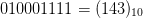 $010001111 = (143)_{10}$.
The first rule could be removed, leaving a consistent system.
However, among Game of Life hobbyists, patterns with fewer living cells
are considered smaller and maintain this for consistency. This does add
some complications to the model which is discussed in the Appendix.
We will append each equation with a number, in the form  $\#i$ indicating that we are interested in the
  $i$th pattern to fit the equation. Thus, the glider becomes
  TeX Source$$\begin{equation*} X\downarrow \rightarrow = X \oplus ^{4}, \#0 \end{equation*}$$ as the smallest pattern which fits the description.
In our discussions of ASC, establishing rules for lexicographical
ordering is important whereas assessing the computational resources
needed to explicitly populate the list is not.
B. Binary Representation
order to use the ASC results, we need to encode the mathematical
representation as a binary sequence. Each symbol is assigned a 5-bit
binary code as specified in Table II. Any valid
formula will be encoded as a binary string using those codes. All such
formulas will be encoded as prefix-free codes.
Firstly, a number of the operations have zero arguments, known as nullary operators. These are listed first in Table II.
Such operations are simply encoded using their 5-bit sequence. Since
they have no arguments, their sequence is completed directly after the
five bits. As noted, a different set of operations could be chosen that
would require a different number of bits to specify. Thus,  $X$ will be encoded as 00000 and
  $W$ will be encoded as 00011. All the nullary operations are trivially prefix free since all have exactly five bits.
An operation that takes a single argument, known as a unary
operation, can be encoded with its 5-bit code followed by representation
of the subexpression. Thus,  $X\uparrow$
can be represented as 01001 00000. Since the subexpression can be
represented in a prefix free code, we can determine the end of it, and
adding five bits to the beginning maintains the prefix-free property.
$X\uparrow$
can be represented as 01001 00000. Since the subexpression can be
represented in a prefix free code, we can determine the end of it, and
adding five bits to the beginning maintains the prefix-free property.
Operations with two arguments, or binary operations, are encoded
using the 5-bit sequence followed by the sequence for the two
subexpressions. So  $X = X \oplus$ can be recorded as 10101 00000 01000 00000.
  $\oplus ^{i}$ can be recorded as 10111 01000 00100. Note that
  $\oplus$
usually takes an argument, but this is not needed when it is used as
the target of a repeat. As with the unary case, the prefix free nature
of the subexpressions allows the construction of the large formula.
$\oplus$
usually takes an argument, but this is not needed when it is used as
the target of a repeat. As with the unary case, the prefix free nature
of the subexpressions allows the construction of the large formula.
The literals in Table II are denoted by the 5-bit code along with an encoding of the integer or pattern. Any positive integer  $n$ can be encoded using
 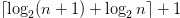 $\lceil \log _{2} (n+1) + \log _{2} n \rceil + 1$ bits, hereafter
  $l(n)$ bits in a prefix free code using the Levenstein code [47]. See Section III-C for a discussion of binary encodings for arbitrary patterns.
To declare there are no more operations to be had, we will use the
five bit sequence, 11111. Simply concatenating all the equations would
not be a prefix-free code since the binary encoding would be a valid
prefix to other codes. After the last equation, 11111 is appended as a
suffix preventing any longer codes from being valid and making the
system prefix free.
To calculate the length of the encoding we add up the following.
- Five bits for every symbol.
 $l(n)$ bits for each number
  $n$ in the equation.
- The length of the bit encoding of any pattern literals.
- Five bits for the stop symbol.
 $l(n)$ bits for the parameters and sequence numbers.
C. Binary Encoding for Patterns
In order to use OASC we need to define the complexity or probability
of the patterns. We would like to define the probability based on the
actual probability of the pattern arising from a random configuration.
We will model the patterns as being generated by a random sequence of
bits.
In order to use a random encoding of bits, we need to define the bit encoding for a Game of Life pattern. Section III-B
contains a definition of an encoding, but it is based on functionality.
The probability of a pattern arising is clearly not related to its
functionality, and thus this measure is not a useful encoding for this
purpose.
There are different ways to define this encoding. We can encode the
width and height of the encoding using Levenstein encoding and each cell
encoded as a single bit indicating whether it is living or not. This
gives a total length of  TeX Source$$\begin{equation*} \alpha (p) = l(p_{w}) + l(p_{h}) + p_{w} p_{h} \end{equation*}$$ where
  $p_{w}$ is the width of the pattern
  $p$ and
  $p_{h}$ is the height of the pattern. We will call this the standard encoding.
However, in many cases patterns consist of mostly dead cells. A lot
of bits are spent indicating that a cell is empty. We can improve this
situation by recording the number of live bits and then we can encode
the actual pattern using less bits  TeX Source$$\begin{equation*}
\beta (p) = l(p_{w}) + l(p_{h}) + l(p_{a}) + \left \lceil \log _{2}
\binom{p_{w} p_{h} }{ p_{a}} \right \rceil \end{equation*}$$ where
TeX Source$$\begin{equation*}
\beta (p) = l(p_{w}) + l(p_{h}) + l(p_{a}) + \left \lceil \log _{2}
\binom{p_{w} p_{h} }{ p_{a}} \right \rceil \end{equation*}$$ where  $p_{a}$ is the number of alive cells. We will call this compressed encoding.
To demonstrate these methods, consider the Gosper gliding gun in Fig. 4. Using the standard encoding this requires 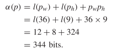 TeX Source$$\begin{align*}
\alpha (p)=&l(p_{w}) + l(p_{h}) + p_{w} p_{h} \\=&l(36) + l(9) +
36 \times 9 \\=&12 + 8 + 324 \\=&344 \textrm {bits.}
\end{align*}$$ Using the compressed encoding requires
TeX Source$$\begin{align*}
\alpha (p)=&l(p_{w}) + l(p_{h}) + p_{w} p_{h} \\=&l(36) + l(9) +
36 \times 9 \\=&12 + 8 + 324 \\=&344 \textrm {bits.}
\end{align*}$$ Using the compressed encoding requires 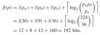 TeX Source$$\begin{align*}
\beta (p)=&l(p_{w}) + l(p_{h}) + l(p_{a}) + \left \lceil \log _{2}
\binom{p_{w} p_{h} }{ p_{a}} \right \rceil \\=&l(36) + l(9) + l(36) +
\left \lceil \log _{2} \binom{324 }{ 36} \right \rceil \\=&12 + 8 +
12 + 160 = 192 ~\textrm {bits}. \end{align*}$$
TeX Source$$\begin{align*}
\beta (p)=&l(p_{w}) + l(p_{h}) + l(p_{a}) + \left \lceil \log _{2}
\binom{p_{w} p_{h} }{ p_{a}} \right \rceil \\=&l(36) + l(9) + l(36) +
\left \lceil \log _{2} \binom{324 }{ 36} \right \rceil \\=&12 + 8 +
12 + 160 = 192 ~\textrm {bits}. \end{align*}$$
The compressed method will not always produce smaller descriptions as
it does here. However, we can use both methods, and simply add an
initial bit to specify which method was being used. Thus, the length of
the encoding for a pattern,  $p$ is then
  TeX Source$$\begin{equation*} P(p) = 1 + \min (\alpha (p), \beta (p))\tag{11}\end{equation*}$$ where the 1 is to account for the extra bit used to determine which of the two methods was used for encoding.
However, we need to determine the Shannon information for a pattern,  $p$. There are two ways to encode each pattern and both need to be considered
  TeX Source$$\begin{equation*} \Pr [X = p] = \Pr [X = p|C]\Pr [C] + \Pr [X = p|\overline {C}]\Pr [\overline {C}] \end{equation*}$$ where
  $X$ is the random variable of the chosen pattern, and
  $C$ is the random event which is true when the compressed encoding is used. Since either method is chosen with 50% probability
 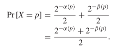 TeX Source$$\begin{align*}
\Pr [X = p]=&\frac {2^{-\alpha (p)}}{2} + \frac {2^{-\beta (p)}}{2}
\\=&\frac {2^{-\alpha (p)} + 2^{-\beta (p)}}{2}. \end{align*}$$
TeX Source$$\begin{align*}
\Pr [X = p]=&\frac {2^{-\alpha (p)}}{2} + \frac {2^{-\beta (p)}}{2}
\\=&\frac {2^{-\alpha (p)} + 2^{-\beta (p)}}{2}. \end{align*}$$
Our primary purpose in this paper is to demonstrate OASC for
functional machines in the Game of Life. However, the process also
serves as a test of the hypothesis that the approximation to the
probability of a pattern and its corresponding information in (11)
arising is reasonably close. Are there features of random Game of Life
patterns that tend to produce additional functionality? If so, we expect
that we will obtain larger than expected values of ASC.
D. Computability
The contextual mathematical formulation thus far developed here for
the Game of Life is less powerful than a Turing complete language. For
example, there is no conditional looping mechanism. The Game of Life itself is Turing complete [48]; however, our equations using the components in Table II
describing the Game of Life are not. There are concepts that cannot be
described using the operations we have defined. A large array of a
billion closely spaced albeit noninteracting blinkers has low KCS
complexity akin to the celebrated low KCS complexity of a repetitive
crystalline structure. A looping or a REPEAT command is required to
capture low KCS complexity bound in such cases. The list in Table II
of course, can be expanded to include these and other cases. However,
the proof on the bound of ASC only requires that the language used to
describe the pattern is prefix-free. Thus, the ASC bounds using the
context in Table II still apply to the language defined here.
In order to use ASC, we must algorithmically derive the machine from
the equations describing it. A program would systematically test all
pattern in order of increasing size while checking whether they pass the
test. We term this program the interpreter. Since the pattern specified
whether it is the first, second, third, etc., pattern to pass the test,
the process can stop and output the pattern once it is reached. Thus, a
constant length interpreter program can derive the pattern from the
equations, and ASC using a standard Turing machine is a constant longer
than the OASC results presented here. If an alternate formulation is
used to describe the pattern, then a different constant would apply as a
different interpreter would be required.
The language used here is motivated in part for simplicity in
understanding. It allows the comparison of the complexity of various
specifications without constants which is difficult in standard KCS
complexity.
Essentially, we have included the interpreter for our formulation as
part of the context. The interpreter has details on the Game of Life,
but not on the nature of patterns in it. This allows the description of
the pattern in the Game of Life without any undue bias toward the
patterns found in the Game of Life.
A. Oscillators
The simplest oscillator is one which does not actually change, i.e., a still life. An example is depicted in Fig. 1. This object can be described as 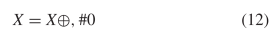 TeX Source$$\begin{equation*} X = X \oplus , \#0\tag{12}\end{equation*}$$
as this is the smallest pattern that can fit the test. There are four
symbols taking 20 bits to describe. There are five bits for the stop
symbol and one bit to describe the sequence number. This gives a total
of 26 bits to describe this pattern. Using standard encoding will
require
TeX Source$$\begin{equation*} X = X \oplus , \#0\tag{12}\end{equation*}$$
as this is the smallest pattern that can fit the test. There are four
symbols taking 20 bits to describe. There are five bits for the stop
symbol and one bit to describe the sequence number. This gives a total
of 26 bits to describe this pattern. Using standard encoding will
require  $l(2) + l(2) + 2\times 2 + 1 = 4+4+4 = 13$. Thus, the ASC is at least
 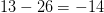 $13 - 26 = -14$ bits of ASC. Since ASC is negative, the pattern is well explained by the stochastic process.
A flip-flop or period two oscillator as depicted in Fig. 2 can be described as  TeX Source$$\begin{equation*} X = X \oplus ^{i}, i = 2, \#0.\tag{13}\end{equation*}$$
This takes six symbols (the repeat counts as a symbol) plus the stop
symbol the parameter and the sequence number. That is a total of
TeX Source$$\begin{equation*} X = X \oplus ^{i}, i = 2, \#0.\tag{13}\end{equation*}$$
This takes six symbols (the repeat counts as a symbol) plus the stop
symbol the parameter and the sequence number. That is a total of  $35 + l(2) + l(0) = 35 + 4 + 1 = 40$ bits. The blinker encoded using standard encoding will take
  $l(1) + l(3) + 3 + 1 = 2 + 5 + 3 + 1 = 11$ bits. The OASC is then
  $11 - 40 = -29$ bits. Again, this pattern fits the modeled stochastic process well.
However, the same pattern could be described as
which has three symbols, and will require 11 bits for the pattern.
The #0 is required, despite there being only one pattern which fits the
equation, for consistency with the search process described in Section III -D. Thus, the length is  $3\times 5 + 5 + l(0) + 11 = 20 + 1 + 11 = 32$ giving at least
 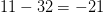 $11 - 32 = -21$
bits of ASC. In fact any pattern can be said to have at least −21 bits
of ASC, because that is the overhead required to simply embed the
pattern in its own description.
$11 - 32 = -21$
bits of ASC. In fact any pattern can be said to have at least −21 bits
of ASC, because that is the overhead required to simply embed the
pattern in its own description.
Simply by changing the value of  $i$ this same construct can describe an oscillator of any period. It will describe the smallest known oscillator of that period. Fig. 53
shows the smallest known oscillators for periods up to nine. Smaller
oscillators than these may exist, but for now we believe these to be the
ones described by the formulation. Table III shows the calculated values of OASC for the various oscillators. The
$i$ this same construct can describe an oscillator of any period. It will describe the smallest known oscillator of that period. Fig. 53
shows the smallest known oscillators for periods up to nine. Smaller
oscillators than these may exist, but for now we believe these to be the
ones described by the formulation. Table III shows the calculated values of OASC for the various oscillators. The  $\Pr [X]$ column derives from experiments on random soups [50]. The missing entries do not appear to have been observed in random trials.
The  $K(X|C)$
for the smallest known oscillator increases slowly as the period
increases. The complexity generally increases, but not always. Caterer
is the first oscillator with a positive amount of ASC. It does appear
out of random configurations but at a rate much lower than the ASC
bound. The ASC bound is violated in only one case, that of the unix
oscillator. This oscillator shows up more often than our assumption
regarding the probabilities would suggest. The pattern has a certain
simplicity to it which is not captured by our metric.
$K(X|C)$
for the smallest known oscillator increases slowly as the period
increases. The complexity generally increases, but not always. Caterer
is the first oscillator with a positive amount of ASC. It does appear
out of random configurations but at a rate much lower than the ASC
bound. The ASC bound is violated in only one case, that of the unix
oscillator. This oscillator shows up more often than our assumption
regarding the probabilities would suggest. The pattern has a certain
simplicity to it which is not captured by our metric.
Any pattern in the Game of Life can be constructed by colliding gliders [46].
The unix pattern can be constructed by the collision of six gliders.
The psuedo-barberpole, the smallest known period five oscillator,
requires 28 gliders. The burloaferimeter, the smallest known period
seven oscillator, requires 27 gliders. The unix pattern requires fewer
gliders to construct than either of the two most similar oscillators
considered here. For its size, the unix pattern is easier to construct
than might be expected.
B. Spaceships
A spaceship is a pattern in life which travels across the grid. It
continually returns back to its original state but in a different
position. The first discovered spaceship was the glider depicted in Fig. 3. We previously showed in (7) that it could be described as  TeX Source$$\begin{equation*} X\downarrow \rightarrow = X \oplus ^{4}, \#0. \end{equation*}$$ This has eight symbols so the length will be
  $5\times 8 + 5 + l(4) + l(0) = 45 + 6 + 1 = 52$. The complexity is 20 and the ASC is at least
  $20 - 52 = -32$
bits. As previously noted, any pattern can be described such that it
has at least −21. This matches the observation that glider often arise
from random configurations.
$20 - 52 = -32$
bits. As previously noted, any pattern can be described such that it
has at least −21. This matches the observation that glider often arise
from random configurations.
As with oscillators we can readily describe the smallest version of a
spaceship. In addition to varying with respect to the period,
spaceships vary with respect to the speed and direction. Speeds are
rendered as fractions of  $c$, where
  $c$
is one cell per iteration. First we will consider spaceships that
travel diagonally like the glider. In general to travel with a speed of
$c$
is one cell per iteration. First we will consider spaceships that
travel diagonally like the glider. In general to travel with a speed of  $c/s$ with period
  $p$ can be described as
  TeX Source$$\begin{equation*} X\downarrow ^{\frac {p}{s}}\rightarrow ^{\frac {p}{s}} = X\oplus ^{p}, \#0.\tag{15}\end{equation*}$$
This describes a spaceship moving down and the right. Due to the
symmetry of the rules of the Game of Life, the same spaceships could all
be reoriented to point in different directions. That would change the
direction of the arrows, but not the length of the description. The
length of this is
TeX Source$$\begin{equation*} X\downarrow ^{\frac {p}{s}}\rightarrow ^{\frac {p}{s}} = X\oplus ^{p}, \#0.\tag{15}\end{equation*}$$
This describes a spaceship moving down and the right. Due to the
symmetry of the rules of the Game of Life, the same spaceships could all
be reoriented to point in different directions. That would change the
direction of the arrows, but not the length of the description. The
length of this is  $5\times 12 +5 + l(\frac {p}{s}) + l(p) + l(0) = 66 + l(\frac {p}{s}) + l(p)$.
Fig. 6 shows the smallest known diagonally
moving spaceships for different speeds. If we assume that these are the
smallest spaceships for these speeds, then (15) describes them. Table IV
shows the ASC for these various spaceships. The glider has negative
ASC, it is simple enough to be readily explained by a random
configuration. The remaining diagonal spaceships exhibit a large amount
of ASC, fitting the fact that they are all complex designs. This is
expected from look at Fig. 6 where the remaining patterns are much larger than the glider.
In addition to the diagonally moving spaceships we can also consider
orthogonally moving spaceships. These move in only one direction, and so
can be described as  TeX Source$$\begin{equation*} X\uparrow ^{\frac {p}{s}} = X\oplus ^{p}, \#0.\tag{16}\end{equation*}$$
The length of this is  $5\times 9 + 5 + l(\frac {p}{s}) + l(p) + l(0) = 51 + l(\frac {p}{s}) + l(p) + l(0)$.
As with the diagonal spaceships, the same designs can be reoriented to
move in any direction. The equation can be updated by simply changing
the arrow. Fig. 7 shows the smallest known spaceship for a number of different speeds. Table V
shows the ASC for the various spaceships. The simplest orthogonal
spaceship, the lightweight spaceship, has negative bits of ASC. This
matches the observation that these spaceships do arise out of random
configurations [51]. The remaining spaceships exhibit significant
amounts of ASC, although not as much as the diagonal spaceships, and are
not reported to have been observed arising at random.
$5\times 9 + 5 + l(\frac {p}{s}) + l(p) + l(0) = 51 + l(\frac {p}{s}) + l(p) + l(0)$.
As with the diagonal spaceships, the same designs can be reoriented to
move in any direction. The equation can be updated by simply changing
the arrow. Fig. 7 shows the smallest known spaceship for a number of different speeds. Table V
shows the ASC for the various spaceships. The simplest orthogonal
spaceship, the lightweight spaceship, has negative bits of ASC. This
matches the observation that these spaceships do arise out of random
configurations [51]. The remaining spaceships exhibit significant
amounts of ASC, although not as much as the diagonal spaceships, and are
not reported to have been observed arising at random.
D. Eaters
Most of time when a glider hits a still life, the still life will
react with the glider and end up being changed into some other pattern.
However, with patterns known as eaters, such as that displayed in Fig. 9,
the pattern “eats” the incoming glider resulting it returning to its
original state. There are two aspects that make it an eater. Firstly, it
must be a still life  TeX Source$$\begin{equation*} X = X \oplus.\tag{18}\end{equation*}$$
Secondly, it must recover from eating the glider
The two equation have a total of 18 symbols, and the glider will require 20 bits to encode. Thus, the total length will be  $5\times 18 + 5 + 20 + l(3) + l(4) + l(4) + l(0) = 5\times 18 + 5 + 20 + 4 + 7 + 7 + 1 = 134$ bits. The complexity of the eater is 29 bits. The OASC is thus
 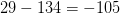 $29 - 134 = -105$ bits. The eater is thus simple enough to be explain by a random configuration.
E. Ash Objects
Within the Game of Life, it is possible to create a random soup of cells and observe what types of objects arise from the soup. The resulting stable objects, still-lifes and oscillators, are known as ash [46]. Experiments have been performed to measure the frequencies of various objects arising from this soup [50]. Fig. 10
shows the ten most common ash objects, together comprising 99.6% of all
ash objects. We observe that these objects are fairly small, and thus
will not exhibit much complexity. The largest bounding box is  $4\times 4$ which will require at most
  $1 + l(4) + l(4) + 16 = 1 + 7 + 7 + 16 = 31$
bits. Describing the simplest still life required 26 bits, leaving at
most 4 bits of ASC. Consequently, none of these exhibit a large amount
of ASC.
$1 + l(4) + l(4) + 16 = 1 + 7 + 7 + 16 = 31$
bits. Describing the simplest still life required 26 bits, leaving at
most 4 bits of ASC. Consequently, none of these exhibit a large amount
of ASC.
We have demonstrated the ability to describe functional Game of Life
pattern using a mathematical formulation. This allows us in principle to
compress Game of Life patterns which exhibit some functionality. Thus,
ASC has the ability to measure meaningful functionality.
We made a simplified assumption about the probabilities of various
pattern arising. We have merely calculated the probability of generating
the pattern through some simply random process not through the actual
Game of Life process. We hypothesized that it was close enough to
differentiate randomly achievable patterns from one that were
deliberately created. This appears to work, with the exception of the
unix pattern. However, even that pattern was less than an order of
magnitude more probable than the bound suggested. This suggests the
approximation was reasonable, but there is room for improvement.
We conclude that many of the machines built in the Game of Life do
exhibit significant ASC. ASC was able to largely distinguish constructed
patterns from those which were produced by random configurations. They
do not appear to have been generated by a stochastic process
approximated by the probability model we presented.
There are many more patterns in the Game of Life which have been
invented or discovered. We have only investigated a sampling of the most
basic patterns. Further investigation of specification in Game of Life
pattern is certainly possible. Our work here demonstrates the
applicability of ASC to the measure of functional meaning.
The authors would like to thank the reviewers’ suggestion of
contrasting our paper with the study of temporal emergence properties of
cellular automata.


